







Archive
12.11.2026


 0
 0
 Touch operator panels Weintek
 Meters-indicators
 Controllers (PID, ON/OFF)
 I/O modules

I/O modules
 Spark protection barrier

Spark protection barrier
 Recorders and archivers

Recorders and archivers
 Meters and converters of electrical network parameters

Meters and converters of electrical network parameters
 Counters, timers, tachometers

Counters, timers, tachometers
 Liquid level indicators and regulators

Liquid level indicators and regulators
 Programmed logical controllers

Programmed logical controllers
 Manual signal transmitters

Manual signal transmitters
 Technological signaling devices

Technological signaling devices
 Power supplies

Power supplies
Codesys PLC controllers
Codesys PLC controllers
 Normalizing converters

Normalizing converters
Galvanic isolation and branching blocks
Galvanic isolation and branching blocks
 Communication interface converters and amplifiers

Communication interface converters and amplifiers
 Analytical instruments

Analytical instruments
 Switching blocks

Switching blocks
Control and protection units
Control and protection units
 GSM communication routers / modems

GSM communication routers / modems
Archive
12.11.2026
Author
Ihor Kravchuk
E-mail: ihorkravchukster@gmail.com
Valerii Dykhnilkin, Microl LLC
E-mail: asutp@microl.ua
The wide range of PID control algorithms implemented in the MIK-51 controller makes it possible to build highly complex multi-loop automatic control systems for a variety of industrial processes.
It is no secret that in practice there are no simple processes, and no simple control loops either. The whole variety of plants cannot be reduced to a single process control template. So a young engineer fresh from university will be shocked to find that much of what control theory textbooks say about control loops is "slightly" different from reality. The engineer first has to learn the basics of how automatic controllers work in real conditions.
Speaking of controllers: the familiar PID controller was invented back in 1910. A method for tuning its parameters was first proposed by Ziegler and Nichols in 1942. Since then, the controller has undergone many changes, giving rise to a whole series of devices whose internal structure differs (sometimes considerably) from that of the ideal PID controller.
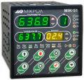
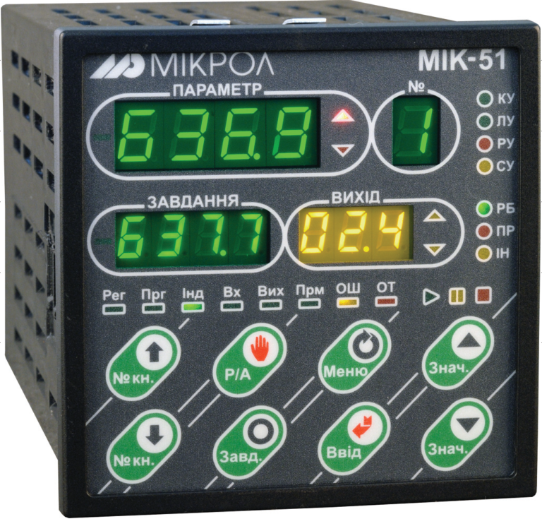
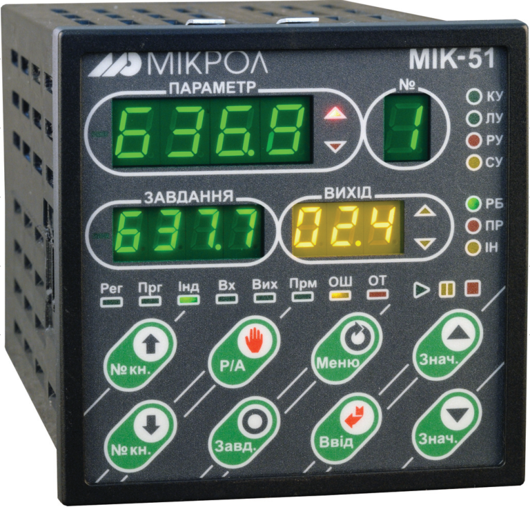
As an example, let us look at the PID controllers in the algorithm library of the MIK-51 universal controller made by Microl (Ivano-Frankivsk). The MIK-51 has 7 PID algorithms in total, so varied that a single controller can be used to build complex multi-loop automatic control systems.
The PID(60) function block (Fig. 1) is a conventional analog PID controller that can operate in 4 modes: manual (RU), local (LU), cascade (KU — when two such blocks are used) and tracking (SU).
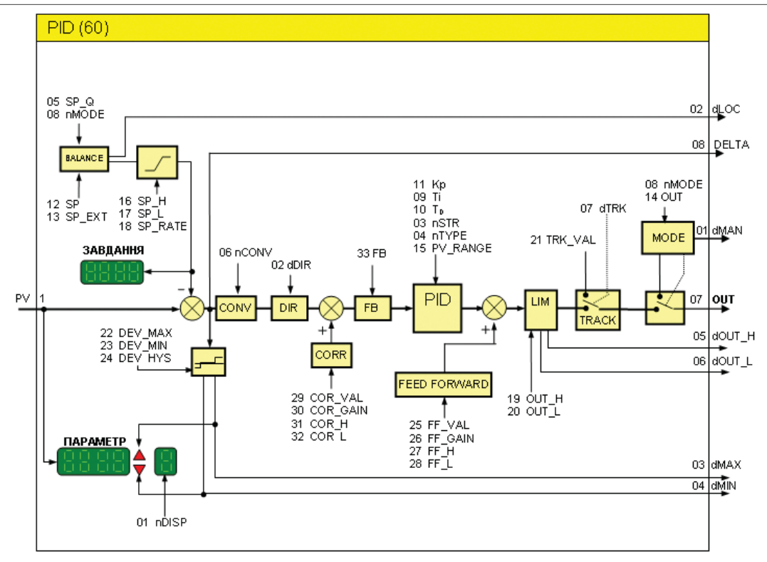
Fig. 1. Structure of the PID(60) function block (tracking mode)
The PID_IMP(62) function block is similar to the previous one but works with a pulse-driven actuator (for example, an MEO). Accordingly, it has additional tuning parameters: minimum pulse duration, actuator travel time, minimum delay between switch-ons and a variable for tracking the actuator position. As with the analog PID controller, two PID_IMP(62) blocks can be combined into a cascade controller.
The PID_CAS(61) block can replace two analog PID blocks connected in cascade, but it is more robust to disturbances and has additional internal protections when parameters approach pre-emergency values. In addition, PID_CAS(61) is tied to a single front panel, which makes it much easier to operate (two PID(60) blocks in cascade would use two front control panels).
The PID_R(90) function block is similar to PID(60) but with a modified mode-switching scheme. It adds MAN, LOC and CAS digital inputs and a setpoint output, which allows control loop programs to switch modes from within the program.
Last on the list (but perhaps first in versatility) are the delta controller function blocks — analog (D_PID(95), Fig. 2) and pulse (D_PID_I(96)). On the one hand, the way delta controllers work is somewhat harder to grasp; on the other, they are universal building blocks from which an automatic control system of any complexity can be assembled. With appropriate tuning, a delta controller can act as any of the controllers above, with additional functionality.
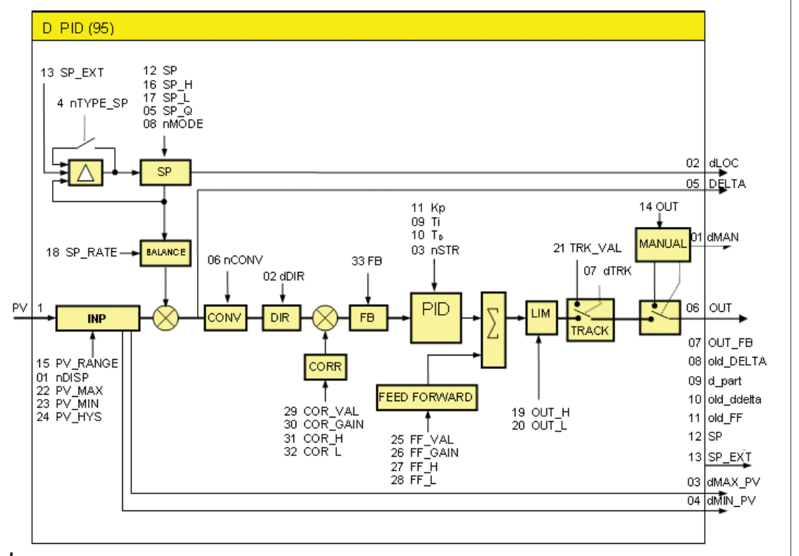
Fig. 2. Structure of the D_PID(95) function block
Fig. 3 shows a cascade control loop built from two D_PID(95) delta controller blocks. At first glance, the scheme looks like a typical cascade loop. But there are several differences. First, such a loop does not have to consist of just two blocks (D-PID-MASTER and D-PID-SLAVE). The structure can be extended both "in length" (cascade and multi-cascade control) and "in width" (parallel control loops, for example when there is one measured variable but two control valves: on the main line and on the bypass).
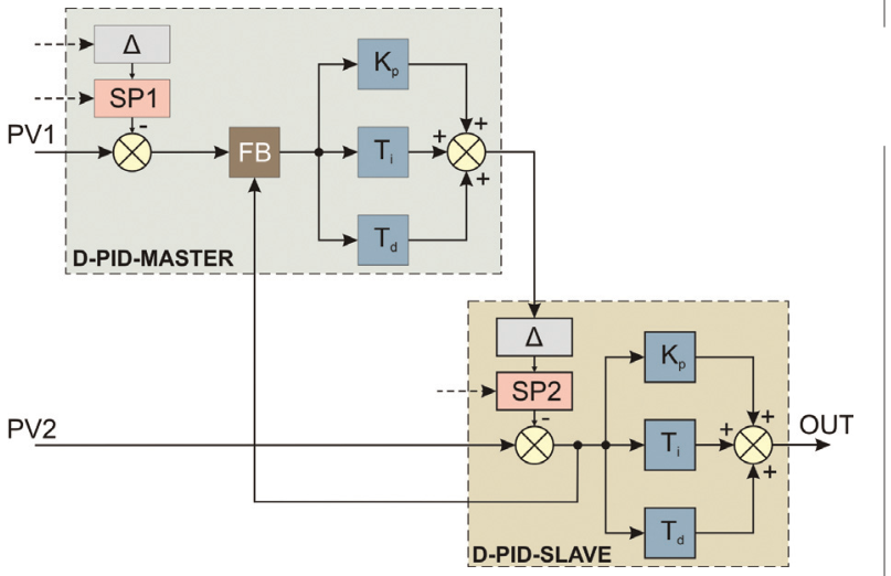
Fig. 3. Structure of a cascade control loop
The next difference is a special Δ block in the controller structure, which adjusts the setpoint according to a defined law. It ensures bumpless setpoint changes for any controller in the cascade (not just the MASTER controller, as in conventional schemes) and also improves the stability of the system as a whole.
Another difference is a nonlinear negative feedback path between the controllers (FB, FeedBack). It considerably increases the system's stability margin and simplifies tuning. By processing the feedback, the controllers monitor themselves when large deviations occur. In addition, the feedback inputs and outputs of the function blocks make it possible to build a multivariable controller on the MIK-51.
Fig. 4 shows a "wide" loop structure with two delta controllers connected in parallel. This loop is used when high control accuracy is needed. The plant has two control valves: one on the main line and one on the bypass (the latter with a much smaller capacity). D-PID-1 works as a normal PID controller and positions the main-line valve. Controller D-PID-2 (responsible for the bypass valve) is connected so that the controlled variable is not fed to its input. Instead, it is tied to the feedback block output of D-PID-1, whose signal goes to the CORR correction block of D-PID-2. By configuring the DIR block of this controller, D-PID-2 can be set to work in phase with D-PID-1 or in antiphase, thereby minimizing possible overshoot in the closed loop.
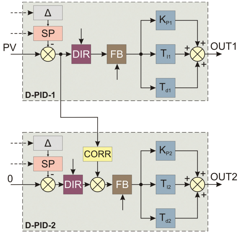
Fig. 4. Structure of a parallel control loop
All PID function blocks in the MIK-51 algorithm library share a number of common units that make them compatible with each other and more versatile. These include:
Switching to tracking mode pauses the controller. It "freezes", storing the proportional (Kp), integral (Ti) and derivative (Td) components of the control action at the moment of switching. When it returns from tracking to local mode, the controller resumes from the stored Kp, Ti and Td values, taking balancing into account.
There are 3 main ways to use tracking mode in automatic control loops. First, it is used in emergencies or abnormal situations. The controller switches to this mode when a logical "1" is applied to the dTRK input of the PID block. The controller output then goes to the safe position set in the TRK_VAL parameter, or tracks the value of that parameter if it is programmed as linked.
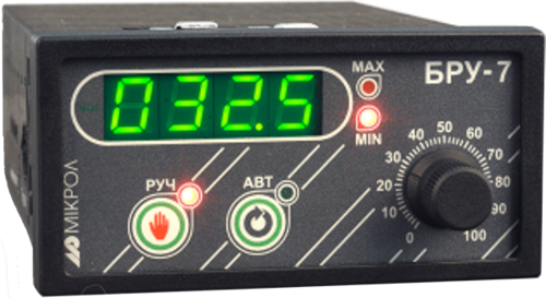
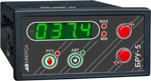
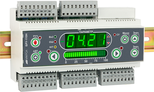
Another use of tracking mode is to follow feedback from the plant. This involves a BRU-10 manual control unit (or -5, -5K1, -7, -7K1) installed locally and inserted into the control signal line between the controller and the actuator. When the BRU unit is in automatic mode, the controller signal goes straight to the actuator. When the BRU unit is switched to local manual control, it generates a digital signal that puts the MIK-51 PID controller into tracking mode. Through the feedback, the PID controller follows the position of the actuator, which is now operated from the BRU front panel. This arrangement ensures bumpless transfer when the BRU unit switches from manual back to automatic.
Yet another use of tracking mode in the MIK-51 is to build a "quantum" controller. The idea of quantum control (control in time intervals) is fairly new, but it is already widely used where conventional PID controllers cannot be applied because of the nature of the process (in particular, where the plant operates in a continuous-cyclic mode).
Such a process is tied directly to a time diagram. First, raw material is loaded into the process vessel; then the required processing takes place, with controllers keeping the parameters within the specified limits. The final stage is unloading the product. Then the cycle repeats.
By switching MIK-51 PID controllers from local mode to tracking and back, high control quality can be achieved, because in each cycle the controller resumes from the state it was in when it was switched to tracking.
In conclusion, everything described above is just one part of what the MIK-51 controller can do.
For more information about the products mentioned in this article, please contact Microl LLC:
+38 (0342) 502-701
+38 (067) 359-70-90
+38 (095) 092-07-28
sale@microl.ua, microl_zbut@microl.ua, zbutmicrol@gmail.com
www.microl.ua
Technical support:
+38 (0342) 502-702
+38 (067) 704-00-29
+38 (095) 302-37-57
support@microl.ua, supmicrol@gmail.com
Originally published in Mir Avtomatizatsii (World of Automation) magazine, June–August 2009.
Open the booklet / download PDF